Overview

The core functionality of pvcaptest is provided by the CapData class, which is a wrapper around two pandas DataFrames, data and data_filtered. The data DataFrame holds the unfiltered data and the data_filtered DataFrame is a copy of the data that the CapData filtering methods modify. reset_filter() can be used to reset the data_filtered DataFrame to the unfiltered data. The fit_regression() method is used to fit the regression equation stored in regression_formula to the filtered data.

Conducting a capacity tests with pvcaptest involves the following steps:

Load data from the plant DAS / SCADA system (load_data()) or from a PVsyst file (load_pvsyst()), returning an instance of CapData.
Review / modify the column_groups attribute as needed.
Use the set_regression_cols() method to set the columns or group of columns to be used in the regression.
When there are multiple sensors for a given measurement, use agg_sensors() to aggregate the data from the sensors.
Use the filtering methods to filter the data.
Calculate reporting conditions.
Use fit_regression() method to fit the regression equation to the filtered data.
Repeat the above steps for the modelled data, except calculating reporting conditions, which should be calculated once from either the measured or simulated data.
Compare the regression results for the measured and modelled data.

Loading Measured Data

Generally, the first step to conducting a capacity test is to load data from the plant DAS / SCADA system. This is done using load_data(), which will return an instance of the CapData class. This function makes a number of assumptions about the data, which are described below. The data to be loaded should be a single file or a collection of files in single directory.

The data is in a comma-separated value (CSV) file(s) (other file tye can be used).
The data is in a “wide” format, with each column representing a different measurement and each row a different time.
The first column of the data contains date time information that can be parsed by pandas.
If loading separate files, the files areall csv files.
If you are loading separate files, the row and column indexes do NOT need to match.

load_data() does a few things in addition to loading the data that are required for functionality of many of the CapData methods like agg_sensors(), loc and floc, and the plotting methods and to clean up minor issues in the raw data:

Note

loc and floc can be used to access data, see Accessing Filtered and Unfiltered Data.

Sorts the data by the datetime index.
Drops any rows where all values in the row are duplicates of the any other row.
Reindexes the data so there are no missing time intervals.
Attempts to group the columns by measurement type based on the column names and store the resulting groupings in the column_groups attribute.
If you provide information about the project site (latitude, longitude, elevation, timezone, racking type, racking orientation) it will add modeled clear sky POA and GHI irradiance to the data DataFrame.

Except for the clear sky modelling, the above describes the default behavior of load_data(), which can be adjusted as needed.

If you are loading data from multiple files and the column headings to match across the files, then load_data() will create attempt to join the data by taking the union of the row and column indexes for all files.

Internally, load_data() uses an instance of the DataLoader class, which is available in the data_loader attribute of the returned CapData instance.

Note

Loading data from filetypes other than CSV is possible by passing a custom function to the file_reader argument of load_data(). Also, the extension needs to be passed as a kwarg, e.g. extension='xlsx'.

Note

If it is necessary to modify the data DataFrame to add columns or convert units, it best to do that immediately after loading the data. Followed by calling reset_filters(), which will overwrite the data_filtered DataFrame with the modified data DataFrame.

Column grouping

As mentioned above, much of the functionality of pvcaptest relies on the groupings of the columns of data by measurement type that is stored in column_groups, which is an instance of the ColumnGroups class, but can also be set to a standard python dictionary. column_groups maps a label for each group to a list of the column headings that are in each group.

For example, the first two groups from the Complete Capacity Test example are shown below:

CapData.column_groups = {
    'irr_poa_pyran': [
        'met1_poa_pyranometer',
        'met2_poa_pyranometer'
    ],
    'irr_poa_ref_cell': [
        'met1_poa_refcell',
        'met2_poa_refcell'
    ],
}

The ColumnGroups class provides some convenient features: nice display of the groupings for review and groups as attributes. Having group id as attributes allows groups of columns to be easily accessed using tab completion in Jupyter notebook.

Due to the very wide range of conventions for naming in DAS / SCADA systems, the default approach to grouping columns often fails to return a satisfactory grouping of the columns. This can be addressed by providing an explicit mapping of column group ids to column names in an external file. To do this the path to the file should be passed to group_columns. Excel, JSON, and YAML files are all options. JSON and Yaml must parse to a python dictionary with keys that are string ids of the groups and values that are lists of column names.

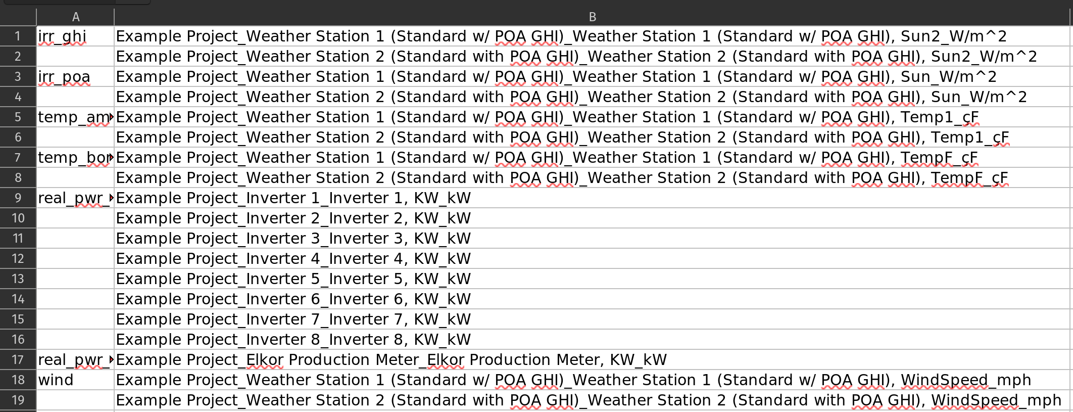
When using an excel file the first column should contain the group ids and the second column should contain all the column headings. The group names do not need to repeated. There should be no header row in the excel file. The most convenient way to create an Excel file specifying the groupings is to run load_data() twice:

Run load_data() with column_groups_template set to True. This will create an Excel file with the column headings in the second column and save it to the same directory as the data files.
Re-order the column headings as necessary and add group ids to the first column.
Run load_data() again with column_groups_template set to False and group_columns set to the path to the Excel.

Screenshot of the excel file loaded in the Concise Example Capacity Test showing the format for defining a column grouping in an Excel file:

../_images/example_excel_column_grouping.png

Note

The column names in the column groups template excel file are sorted alphabetically after reversing the names, so names with the same ending are grouped together. This is often a good starting point for grouping the columns, but it is not always correct, so review carefully!

Dashboard

The plot() method of CapData objects will create a Panel dashboard that can be used to explore timeseries plots of the data.

The dashboard contains three tabs: Groups, Layout, and Overlay.

Groups Tab

The first tab, Groups, presents a column of plots with a separate plot overlaying the measurements for each group of the column_groups attribute. The groups plotted are defined by the default_groups argument. This is the default tab when the dashboard is first opened.

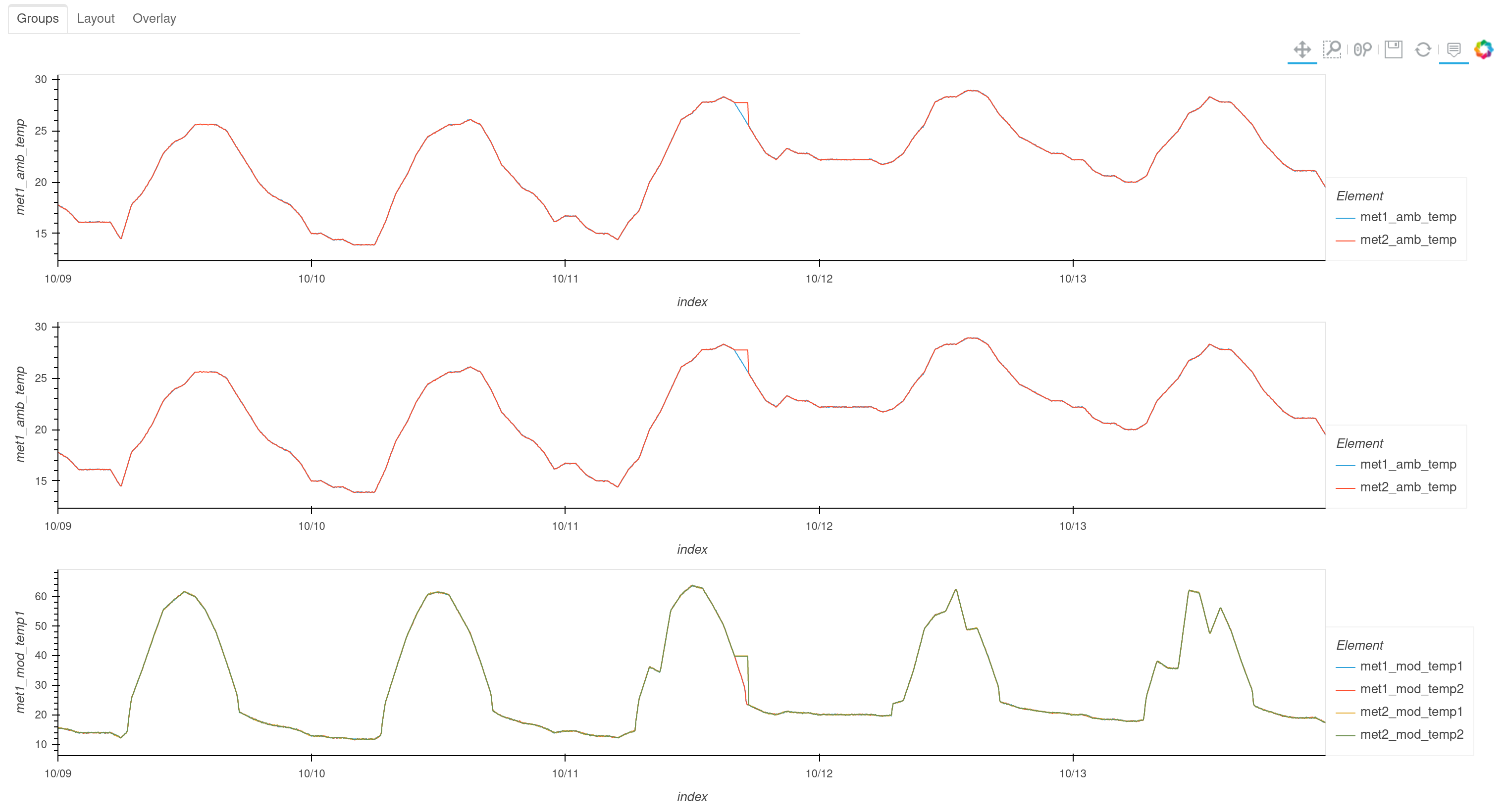
The default_groups argument can be used to specify which groups to plot by passing a list of regular expressions which are used to search the keys of the column_groups attribute. The default list of regular expressions attempts to create the following plots:

Metered power and sum of inverter power, group name is “inv_sum_mtr_pwr”
Inverter power output - group id must contain “real”, “pwr”, “inv”
Metered power output - group id must contain “real”, “pwr”, “mtr”
GHI irradiance
Modeled clear sky POA irradiance
Modeled clear sky GHI irradiance
Ambient temperature and BOM temperature - group name is “temp_amb_bom”

The groups names inv_sum_mtr_pwr and temp_amb_bom are not keys from column_groups, but are created from the dictionary keys of the combine argument. These labels are for combinations of groups from the column_groups attribute. The combine argument can be used to create these combined groups by passing a dictionary of group names and regular expressions. The regular expressions are used to identify groups from column_groups and individual tags (columns) of data to combine into new groups. The dictionary keys are strings which will be used as the names of new groups. Values should be either a string or a list of two strings. If a string, the string is used as a regex to identify groups to combine. If a list, the first string is used to identify groups to combine and the second is used to identify individual tags (columns) to combine.

See the parse_combine() and find_default_groups() functions for more details.

The Layout and Overlay tabs provide the same functionality of combining and selecting groups to be plotted on the Groups tab through a GUI without needing to write regular expressions.

Layout Tab

The Layout tab allows creating a column of plots like the Groups tab by selecting groups from the list.

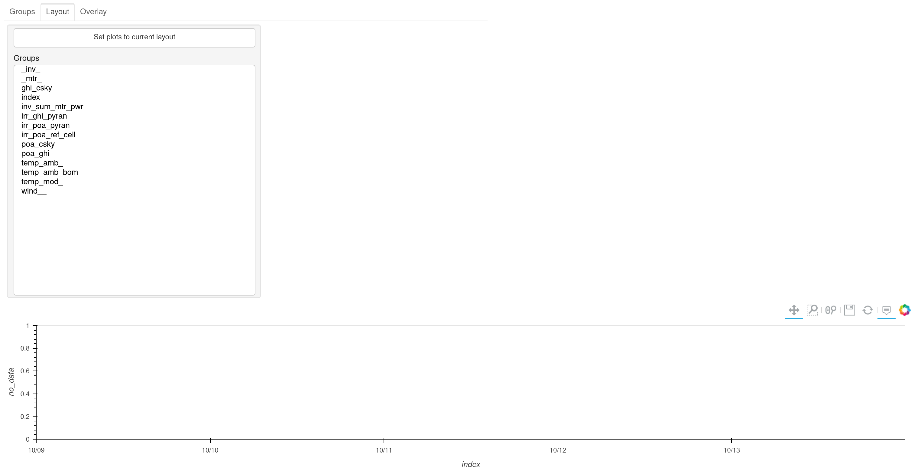
The button labeled “Set plots to current layout” above the list of groups can be used to replace the figure shown on the Groups tab with the current figure on the Layout tab. This will save a plot_defaults.json file in the current working directory that will be used to set the default groups for the Groups tab when the plot() method is called. You will need to rerun the plot method to see the new defaults.

Note

The plots_defaults.json file will override the default_groups argument. If you want to use the default_groups argument, you will need to delete the plot_defaults.json file.

Overlay Tab

The Overlay tab allows picking a group or any combination of individual tags to overlay on a single plot similar to the functionality of the combine argument.

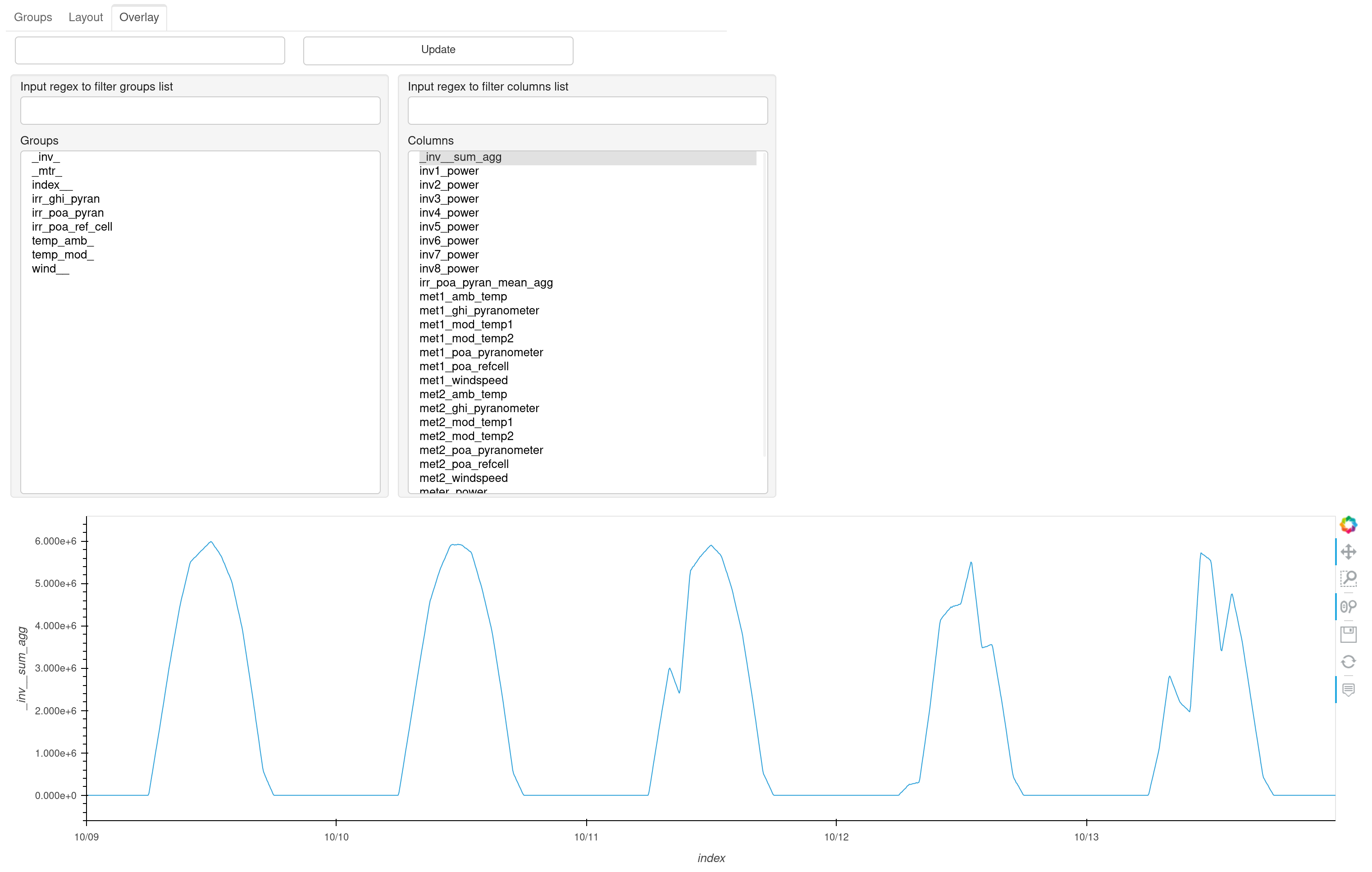
The list of groups and tags can be filtered using regular expressions. The text box at the top left of the tab is used to provide a label for the current overlay, which can be added to the list on the Layout tab by clicking the Update button.

Identifying Regression Data

To perform the regression pvcaptest uses statsmodels, which in turn relies on patsy to simplify specifying regression equations.

By default the ASTM E2848 regression equation is defined in the regression_formula attribute:

'power ~ poa + I(poa * poa) + I(poa * t_amb) + I(poa * w_vel) - 1'

Patsy and Statsmodels expect to find columns with the power, poa, t_amb, and w_vel headings in the DataFrame passed to fit the regression. Rather than requiring those headings to be in the data DataFrame, pvcaptest requires the user to specify which columns or group of columns are to be used in the regression in regression_cols. The set_regression_cols() method can used to identify column headings or column group ids (column_groups keys). Or regression_cols can be set to a dictionary mapping the regression terms defined in the regression_formula to the column headings or column_groups id.

The ability to map a regression term to a group of columns is useful when there are multiple sensors for a given measurement, as described in the next section.

Aggregating Sensors

agg_sensors() can be used to aggregate data from multiple sensors into a single column. This is useful when there are multiple sensors for a given measurement. Any combination of groups of columns and aggregation functions can be passed. By default the groups of columns assigned to the power, poa, t_amb, and w_vel keys in the regression_cols attribute are aggregated by summing the power and averaging the POA irradiance, ambient temperature, and wind speed columns.

agg_sensors() adds the resulting aggregated columns to the data and data_filtered dataframes. If regression_cols included a group of columns that was aggregated, regression_cols is updated to map the regression term to the aggregated column.

For example, if the regression_cols attribute was set to the following:

CapData.regression_cols = {
    'power': 'real_pwr_mtr',
    'poa': 'irr_poa',
    't_amb': 'temp_amb',
    'w_vel': 'wind',
}

Where irr_poa, temp_amb, and wind are the ids of groups of columns in column_groups.

When agg_sensors is called with the default arguments, regression_cols is updated to the following:

CapData.regression_cols = {
    'power': 'real_pwr_mtr',
    'poa': 'irr_poa_mean_agg',
    't_amb': 'temp_amb_mean_agg',
    'w_vel': 'wind_amb_mean_agg',
}

where irr_poa_mean_agg, temp_amb_mean_agg, and wind_amb_mean_agg are the ids of the aggregated columns in data and data_filtered and these columns will be used when fitting the regression.

Accessing Filtered and Unfiltered Data

The methods loc and floc can be used to access columns of data from the data and data_filtered DataFrames, respectively.

Any column heading of the data DataFrame, group id from column_groups, or regression term from regression_cols can be passed to loc or floc. Or, a list with any combination of these identifiers can be passed.

Filtering

The CapData class provides a variety of methods for filtering as described in ASTM E2848. These methods are all begin with “filter_” and are well described in the docstrings of each method.

Running filters removes data from data_filtered. Each subsequent filtering method called will be applied to data_filtered, so the overall filtering is cumulative.

reset_filter() method can be used to reset the data_filtered DataFrame to the unfiltered data.

The get_summary() method will return a summary dataframe showing the number of rows in the data_filtered DataFrame before and after each filter was applied, the name of the each filter, and the arguments passed when calling each filter.

Reporting conditions

rep_cond() can be used to calculate the reporting conditions. The reporting conditions are calculated for columns mapped to the regression_col terms poa, t_amb, and w_vel and are stored in the rc attribute.

Currently there is not functionality to calculate reporting conditions for other regression terms for cases where the default regression formula has been changed. But, the reporting conditions can be calculated manually and assigned to the rc attribute as a dataframe.

The “Reporting Conditions and Predicted Capacities” example demonstrates the reporting condition functionality in more detail.

Fitting Regressions

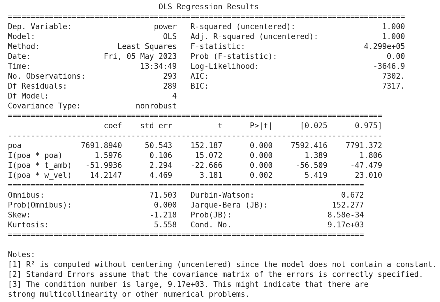
fit_regression() is used to fit the regression equation stored in regression_formula to the filtered data. The statsmodels regression results are stored in the regression_results attribute.

By default a summary showing the results of the regression is printed, similar to below:

Results

After loading, filtering and regressing measured and simulated data in two separate instances of CapData, the results can be compared using the captest_results_check_pvalues(). This will provide a summary of the predicted power using the regression coefficients of each CapData instance and the reporting conditions.

The results function will check and warn for potential issues:

The regression equations in the two CapData instances are different.
Both CapData instances have reporting conditions.

See the Example Capacity Test, for example usage of the results function.

The results from that example display as follows:

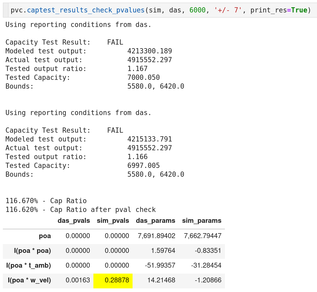
By default the results will be calculated twice. The second calculation will set the regression coefficient for any term where the p-value is greater than 0.05 to zero before calculating the predicted power. These high p-values are highlighted in yellow as shown in the above example for the wind speed regression term of the simulated data.